Kernel Smoother
Functions
Coefficients-Based Smoother
- kerch.method.smoother(coefficients: Tensor, observations: Tensor, num: int | str = 'all') Tensor[source]
Returns a weighted sum of the observations by the coefficients.
\[\mathtt{out}_{i,j} = \frac{\sum_l\mathtt{weights}_{i,l} * \mathtt{observations}_{l,j}}{\sum_l\mathtt{weights}_{i,l}}.\]- Parameters:
coefficients (torch.Tensor [num_points, num_observations]) – coefficients used in the smoother.
observations (torch.Tensor [num_observations, dim_observations]) – observation corresponding to each weight dimension.
num (int or str, optional) – Number of closest points to be used. Either an integer representing the number or the string
'all'. Defaults to'all'.
- Returns:
Weighted observations
- Return type:
torch.Tensor [num_points, dim_observations]
Kernel Smoother
- kerch.method.kernel_smoother(domain: Tensor, observations: Tensor, num: int | str = 'all', kernel_type: str = 'rbf', **kwargs) Tensor[source]
Smoothens the function \(f(\mathtt{domain}_{i,:}) = \mathtt{observation}_{i,:}\) with weights defined as a kernel on the domain.
\[\mathtt{out}_{i,j} = \frac{\sum_l k\left(\mathtt{domain}_{i,:},\mathtt{domain}_{l,:}\right) * \mathtt{observations}_{l,j}}{\sum_l k\left(\mathtt{domain}_{i,:},\mathtt{domain}_{l,:}\right)}.\]The kernel is defined as in
kerch.kernel.factory().- Parameters:
domain (torch.Tensor [num_observations, dim_domain]) – domain corresponding to each observation.
observations (torch.Tensor [num_observations, dim_observations]) – observation corresponding to each domain entry.
num (int or str, optional) – Number of closest points to be used. Either an integer representing the number or the string
'all'. Defaults to'all'.kernel_type (str, optional) – Type of kernel chosen. For the possible choices, please refer to the Factory Type column of the Kernel Module documentation. Defaults to
kerch.DEFAULT_KERNEL_TYPE.**kwargs (dict, optional) – Arguments to be passed to the kernel constructor, such as sample or sigma. If an argument is passed that does not exist (e.g. sigma to a linear kernel), it will just be neglected. For the default values, please refer to the default values of the requested kernel.
- Returns:
Smoothed function \(f\) according to kernel \(k\).
- Return type:
torch.Tensor [num_observations, dim_observations]
Example
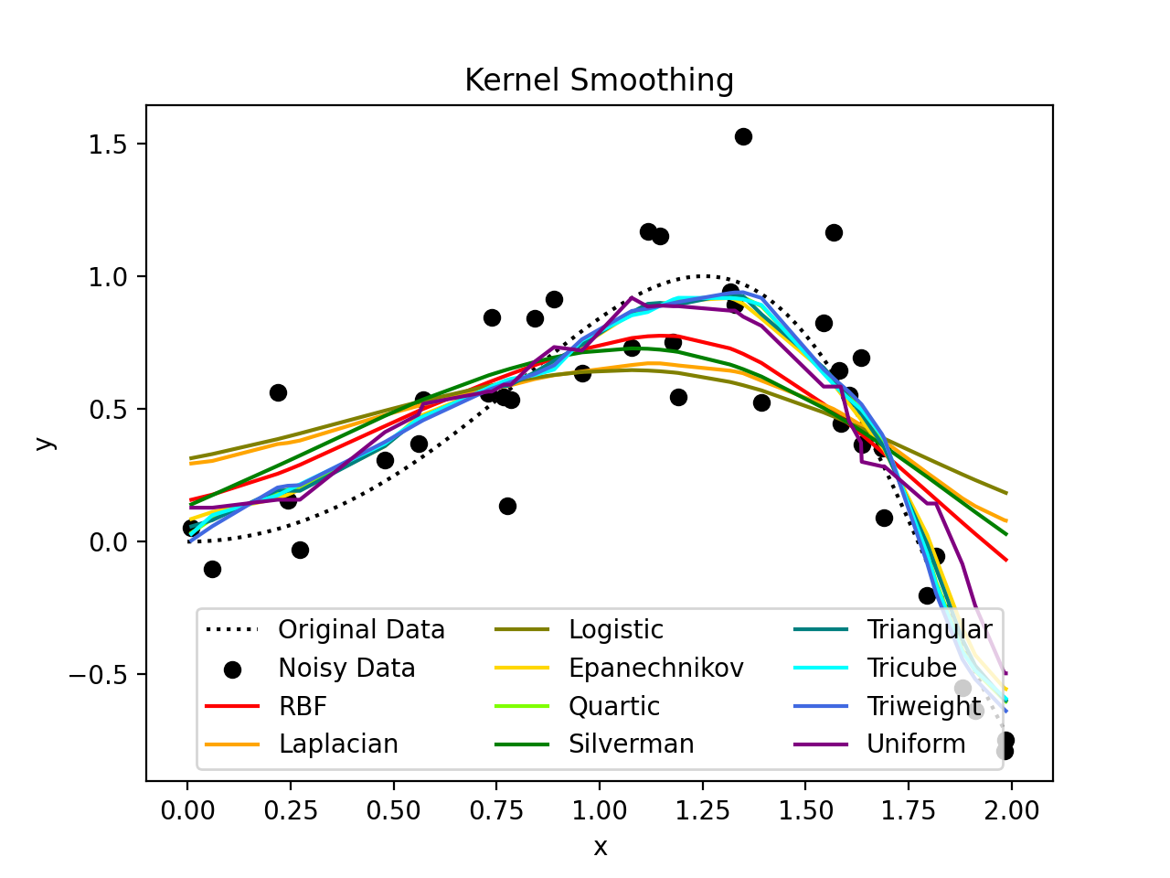
Different Kernels, Same Bandwidth
As we can see in the following example, different kernels have different behaviors. They all use the same bandwidth as without specification, the bandwidth is based on the distance matrix which is here the same for all as they are all based on the same domain. The same bandwidth is not always appropriate for different kernels.
import kerch
import torch
from matplotlib import pyplot as plt

# data
fun = lambda x: torch.sin(x ** 2)

x_equal = torch.linspace(0, 2, 100)
x_nonequal = 2 * torch.sort(torch.rand(40)).values

y_original = fun(x_equal)
y_noisy = fun(x_nonequal) + .2 * torch.randn_like(x_nonequal)

plt.plot(x_equal, y_original, label="Original Data", color="black", linestyle='dotted')
plt.scatter(x_nonequal, y_noisy, label="Noisy Data", color="black")

# kernels
kernels = [('RBF', 'red'),
           ('Laplacian', 'orange'),
           ('Logistic', 'olive'),
           ('Epanechnikov', 'gold'),
           ('Quartic', 'chartreuse'),
           ('Silverman', 'green'),
           ('Triangular', 'teal'),
           ('Tricube', 'cyan'),
           ('Triweight', 'royalblue'),
           ('Uniform', 'purple')]

# kernel smoother
for name, c in kernels:
    y_reconstructed = kerch.method.kernel_smoother(domain=x_nonequal, observations=y_noisy, kernel_type=name.lower())
    plt.plot(x_nonequal, y_reconstructed, label=name, color=c)

# plot
plt.title('Kernel Smoothing')
plt.xlabel('x')
plt.ylabel('y')
plt.legend(loc='lower center', ncol=3)
(Source code, png, hires.png, pdf)
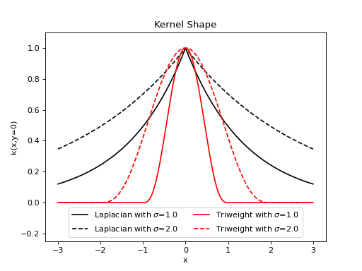
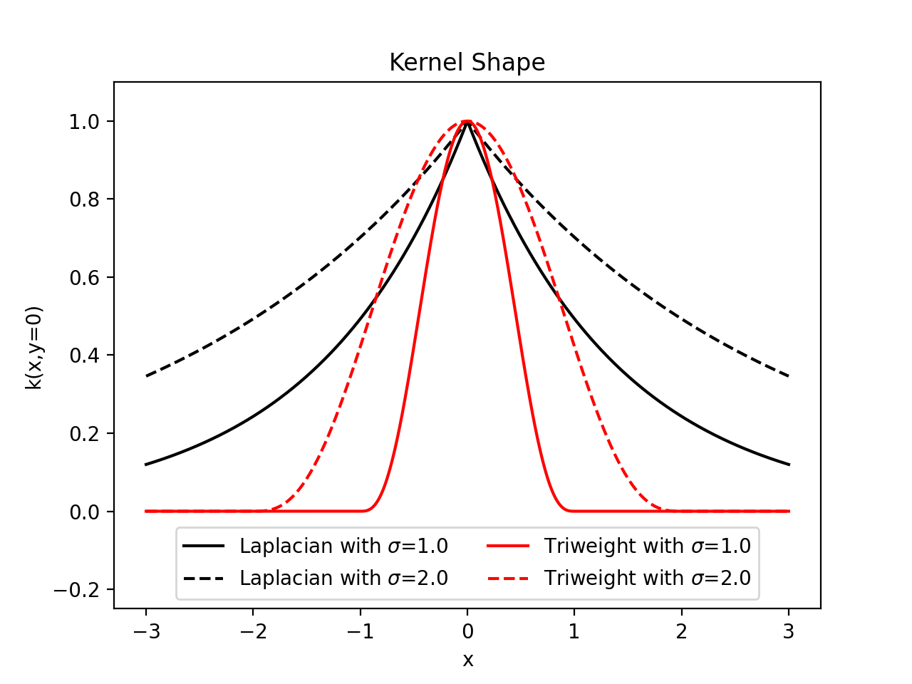
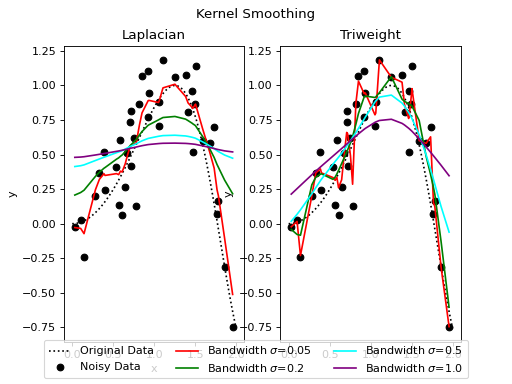
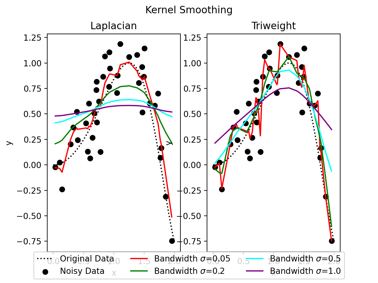
Same Kernels, Different Bandwidths
In this example, we show how two different kernels react differently based on the prescribed bandwidth. We will
consider two kernels, the Laplacian with a very heavy tail and the very restricted
Triweight. We can first have a view at their respective shapes.
import kerch
import torch
from matplotlib import pyplot as plt

# domain
x = torch.linspace(-3, 3, 500)

# define the kernels
k_l1 = kerch.kernel.Laplacian(sample=x, sigma=1)
k_l2 = kerch.kernel.Laplacian(sample=x, sigma=2)
k_t1 = kerch.kernel.Triweight(sample=x, sigma=1)
k_t2 = kerch.kernel.Triweight(sample=x, sigma=2)

# plot the shapes
plt.plot(x, k_l1.k(y=0).squeeze(), label=f"Laplacian with $\sigma$={k_l1.sigma}", color='black')
plt.plot(x, k_l2.k(y=0).squeeze(), label=f"Laplacian with $\sigma$={k_l2.sigma}", color='black', linestyle='dashed')
plt.plot(x, k_t1.k(y=0).squeeze(), label=f"Triweight with $\sigma$={k_t1.sigma}", color='red')
plt.plot(x, k_t2.k(y=0).squeeze(), label=f"Triweight with $\sigma$={k_t2.sigma}", color='red', linestyle='dashed')

# annotate the plot
plt.title('Kernel Shape')
plt.xlabel('x')
plt.ylabel('k(x,y=0)')
plt.ylim(-.25, 1.1)
plt.legend(loc='lower center', ncol=2)
(Source code, png, hires.png, pdf)

import kerch
import torch
from matplotlib import pyplot as plt

# data
fun = lambda x: torch.sin(x ** 2)

x_equal = torch.linspace(0, 2, 100)
x_nonequal = 2 * torch.sort(torch.rand(40)).values

y_original = fun(x_equal)
y_noisy = fun(x_nonequal) + .2 * torch.randn_like(x_nonequal)

# plot
fig, axs = plt.subplots(1, 2)
for ax in axs.flatten():
    ax.plot(x_equal, y_original, label="Original Data", color="black", linestyle='dotted')
    ax.scatter(x_nonequal, y_noisy, label="Noisy Data", color="black")
    plt.title('Kernel Smoothing')
    ax.set_xlabel('x')
    ax.set_ylabel('y')

# kernel smoother
sigmas = [(0.05, 'red'),
          (0.2, 'green'),
          (0.5, 'cyan'),
          (1.0, 'purple')]
for s, c in sigmas:
    y_laplacian = kerch.method.kernel_smoother(domain=x_nonequal, observations=y_noisy, kernel_type='laplacian', sigma=s)
    y_triweight = kerch.method.kernel_smoother(domain=x_nonequal, observations=y_noisy, kernel_type='triweight', sigma=s)
    axs[0].plot(x_nonequal, y_laplacian, color=c, label=f"Bandwidth $\sigma$={s}")
    axs[1].plot(x_nonequal, y_triweight, color=c)

# plot
fig.suptitle('Kernel Smoothing')
axs[0].set_title('Laplacian')
axs[1].set_title('Triweight')
fig.legend(*axs[0].get_legend_handles_labels(), loc='lower center', ncol=3)
(Source code, png, hires.png, pdf)
